Abstract

Machine learning is indispensable in today's society, revolutionizing industries, driving innovation, and empowering intelligent decision-making processes across diverse fields, from healthcare and finance to transportation and entertainment. One of the main components of a basic model is loss function which serves as a metric to quantify the disparity between predicted and actual outcomes, guiding the optimization process in machine learning models. The paper looks into the loss function for regression and classification problem.

Introduction:

In the intricate landscape of machine learning, loss functions serve as guiding beacons, illuminating the path toward optimal model performance. Within the realm of neural networks, understanding the nuances of loss functions is paramount, as they intricately connect the abstract architecture of artificial intelligence to the fundamental workings of the human brain. Neural networks, inspired by the complex web of neurons in the brain, mimic the interconnectedness and adaptability of their biological counterparts. Just as neurons relay signals through synapses, neural networks transmit information through interconnected layers, each processing data to extract meaningful patterns. At the heart of this computational network lies the loss function - a critical component that quantifies the disparity between predicted and actual outcomes. This paper explores the complexity of loss functions. It delves into the concept of loss functions for regression and classification problems in machine learning, which are essential in machine learning algorithms. It explains their significance, intricacies, and impact. From the rudimentary concepts to the forefront of research, the paper delves into the multifaceted world of loss functions for task-specific applications.

Supervised Learning

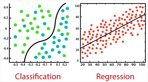
Supervised learning is a type of machine learning algorithm that is given a data set and the correct output, with the idea that there is a relationship between the input and the output. Supervised learning is a machine learning algorithm that involves training a model on a dataset labelled with the correct output. The goal is to find a relationship between the input and the output. Supervised learning can address two types of problems: regression and classification. In regression problems, the model tries to predict a continuous output, such as the price of a house, based on its square footage. On the other hand, in classification problems, the objective is to predict a discrete output, such as whether a patient's tumour is malignant or benign. Classification can also be used in banking to predict the likelihood of default based on variables such as credit history, outstanding loans, and investment details. Similarly, binary classification can be applied to determine whether an email is spam or not based on features like the email's content, sender, and attachments. Multi-class classification can be used to predict the genre of a movie based on its plot summary, actors, and director, where the classes might include action, comedy, or drama used to solve problems that are either associated with "Regression Problems" or "Classification problem" :

• In a regression problem, the model tries to predict results within a continuous output. For example, a regression algorithm is used to predict the price of a house based on its square footage.

• In a classification problem, we are trying to predict results in a discrete output. Classification problem are the one where a bank can use various input variables such as credit history, outstanding loans, and investment details to predict loan default likelihood. Similarly, binary classification can be employed to determine whether an email is spam or not spam based on features like the email's content, sender, and attachments. There are two 2 classes in this situation, it is either "Yes" or "No". In contrast, multi-class classification could involve predicting the genre of a movie based on its plot summary, actors, and director. The classes might include action, comedy, drama, etc. This type of problem, whether binary or multi-class, falls under the "Classification Problems" category.

Source:https://www.datacamp.com/blog/supervised-machine-learning

Unsupervised Learning

Unsupervised learning is a form of machine learning that focuses on identifying patterns within a dataset and organizing individual instances into corresponding categories. These algorithms are unsupervised because the patterns that may or may not exist in a dataset are not informed by a target and are left to be determined by the algorithm [Raximov, Kuvandikov and Dilmurod, 2022]. Unsupervised learning uses datasets with no labels and is typically applied to build a concise representation of the data to derive imaginative content from it. Typical tasks in unsupervised learning include clustering, dimensionality reduction, and density estimation.

1. Clustering: Clustering algorithms group similar data points together into clusters based on some similarity measure. Examples of clustering algorithms include K-means clustering, hierarchical clustering, and DBSCAN.
2. Dimensionality Reduction: Dimensionality reduction techniques aim to reduce the number of features or dimensions in the data while preserving its essential characteristics. Principal Component Analysis (PCA) and t-distributed Stochastic Neighbor Embedding (t-SNE) are popular dimensionality reduction methods.
3. Density Estimation: Density estimation techniques model the underlying probability distribution of the data. Gaussian Mixture Models (GMMs) and kernel density estimation are examples of density estimation methods.

Reinforcement Learning

Reinforcement Learning is a type of learning that may be considered a combinational form of supervised and unsupervised learning. Reinforcement learning draws inspiration from principles of learning and decision-making observed in biological systems. Making mistakes is a standard part of learning. Humans pick up new skills through experimentation and observation of results. In reinforcement learning, an agent aims to match the predicted value with the expected value. This concept can be illustrated through an example where animals receive a juice reward when they press a lever in response to a cue signal (CS), such as a small light turning on. An agent has to learn on the basis of reward signals from the environment rather than explicit demonstration, as is the case in 'supervised learning.' [Jensen, 2023]. Comparably, RL agents investigate various behaviours in their surroundings and gain knowledge from the benefits or drawbacks that arise. Here the learning machine does some action on the environment and gets a feedback response from the environment. The learning system grades its action good (rewarding) or bad (punishable) based on the environmental response and accordingly adjusts its parameters [Dongare, Kharde and D.Kachare, 2008]. Reinforcement learning tasks can be categorized into different types:

1. Episodic Tasks: These are tasks with a clear start and end point, where the agent interacts with the environment for a finite number of steps (episodes). Examples include playing chess or navigating a maze.
2. Continuing Tasks: Tasks where the agent interacts with the environment indefinitely, with no fixed endpoint. The goal is often to maximize long-term rewards. Examples include controlling a robotic arm or managing a stock portfolio.

What are artificial neural networks?

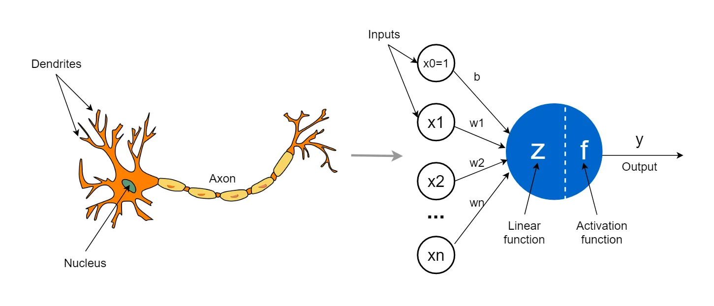
An artificial neural network (ANN) is a computational system that is designed to mimic the structure and function of the human brain. It is a complex network of interconnected processing nodes or artificial neurons, which work together to process and analyze complex information. These artificial neurons are designed to operate similarly to biological neurons in the human brain. The computations of the brain are done by a highly interconnected network of neurons, which communicate by sending electric pulses through the neural wiring consisting of axons, synapses and dendrites [Krogh, 2008]. Just the the brain, the neurons of the artifical neural network allow the network to learn from input data and adjust its connections and weights to improve its accuracy and predictive capabilities.

ANNs have been applied in various fields, including image and speech recognition, natural language processing, and predictive analytics. They have been used to solve complex problems such as language translation, speech recognition, image and video analysis, and financial forecasting. ANNs are ideal for these tasks as they can learn and adapt to new data, making them a powerful tool for solving complex problems in various domains. The mathematical foundations of ANNs are rooted in linear algebra, calculus, and statistics. The design and training of ANNs require careful consideration of these mathematical principles. The network's architecture, activation functions, learning algorithms, and optimization techniques are crucial in determining its performance. The ability of ANNs to learn and adapt to new data makes them a powerful tool for solving complex problems in various domains. There are 4 main components of the a simple machine learning algorithm :

1. Data
2. Back Propagation
3. Forward Pass
4. Loss Function

The focus the paper is the loss function for regression and classification.

Data

Datasets are the very fundamental part of a neural network. They act as a backbone for the neural network to learn/recognize the patterns. Datasets provide the raw material for feature selection and engineering. Features are the variables or attributes used to make predictions with machine learning models. Datasets allow practitioners to identify relevant features, create new features, and preprocess data to improve model performance.

By analyzing datasets, developers can gain insights into the relationships between different features and their impact on the outcome. This understanding helps select the most informative features and design effective machine learning models. Additionally, datasets enable practitioners to assess the quality of the data, handle missing values, and apply necessary transformations for better prediction accuracy. Additionally, datasets serve as benchmarks for comparing the performance of different machine-learning algorithms and techniques. The quality and size of the training samples are crucially important for a successful classification. The more representative samples introduced to a classification process, the more accurate and reliable results can be produced.[Kavzoglu, 2009]. Hence, a reliable, accurate, and relevant problem dataset is the stepping stone for a good neural network.

Forward Pass

A forward pass propagates input data through the network to compute the output. During a forward pass, the input data is passed through the network layer by layer, with each layer applying transformations to the data until the final output is generated. Here is how the forward pass typically works in a neural network:

1. Input Data: The process begins with providing input data to the model. Depending on the model's architecture and the training/inference setup, this input data could be a single or batch of data points.
2. Propagation through Layers: The input data is propagated through the layers of the neural network. Each layer performs a series of operations on the input data, typically involving weighted sums and activation functions.
3. Weighted Sum: The input data is multiplied by weights in each layer, representing the model parameters learned during training. The weighted sum of the input data and the weights is computed.
4. Activation Function: After the weighted sum, an activation function is applied to introduce non-linearity into the model. Common activation functions include ReLU, sigmoid, and tanh.

The output of the last layer in the network serves as the input to the next layer, and this process continues until the data passes through all the layers of the network. The network's final output, which could be a single value (in regression tasks) or a probability distribution over classes (in classification tasks), is generated.

Back Propagation

Backpropagation, or backward propagation of errors, is an algorithm designed to test for errors working back from output nodes to input nodes. It is an important mathematical tool for improving the accuracy of predictions in data mining and machine learning. Essentially, backpropagation is an algorithm used to quickly calculate derivatives in a neural network, which are the changes in output because of tuning and adjustments. [Hashemi-Pour, Zola and Vaughan, n.d.]. Back propagation algorithm works by iteratively adjusting the weights of connections between neurons to minimize the difference between the predicted output and the network's actual output. This process involves two main steps: forward propagation and backward propagation. During forward propagation, input data is passed through the network, layer by layer, to generate predictions. Then, during backward propagation, the error or loss between the predicted and actual outputs is calculated, and this error is propagated backward through the network to update the weights using gradient descent optimization. By computing the gradient of the loss function with respect to each weight in the network, backpropagation allows the network to learn from its mistakes and improve its performance over time. It is a crucial component in training deep learning models and has enabled significant advancements in various fields, including computer vision, natural language processing, and robotics.

Loss Function

The loss function, also known as the cost function or error function, is a mathematical function that measures how closely a model's predictions match the true labels or values in the training data. The model's performance is measured by the loss function, which computes the difference between the goal value and the anticipated output of the model. For this reason, loss functions are a crucial element in the AI model. Selecting a suitable loss function and performance metric is crucial for achieving good performance in deep learning tasks [Terven et al., 2023]. Loss functions optimize the model's parameters during training. Do not confuse loss function to performance metrics." Here is the difference between the loss function and performance metric.

Loss Function	Performance Metrics
loss functions optimize the model’s parameters during training	performance measures assess the model's effectiveness following training.
Loss function is dependant on the model’s architecture and the specific task	less dependent on the model’s architecture and can be used to compare different models or configurations of a single mode
It is challenging to interpret as their values are often arbitrary and depend on the specific task and data.	Performance metrics are more interpretable as they are used across different tasks.

Properties of Loss Function

The loss functions have a series of properties that need to be considered when selected for a machine learning:

1. Convexity: "Convexity is a key feature, since the local minima of convex function is also the global minima" [Ciampiconi et al., n.d.] . Convex loss functions are favoured due to their ease of optimization using gradient-based methods.
2. Differentiability: The differentiability of a loss function for model parameters refers to the ability to calculate derivatives continuously and consistently. This property is crucial for effectively employing gradient-based optimization techniques. Essentially, if the loss function is differentiable, small changes in the model's parameters result in predictable changes in the loss, enabling efficient optimization through gradient descent methods.
3. Smoothness: The loss function must have a continuous gradient without abrupt spikes or changes.
4. Robustness: A minimal number of extreme values should not impact the loss functions; instead, they should be able to manage outliers.
5. Multimodality: A loss function with more than one global minimum is considered multimodal. When a model is required to learn several data representations, multimodal loss functions may be helpful.
6. Sparsity: The model will produce outputs with fewer active elements if the loss function incentivizes sparsity. This feature proves advantageous in high-dimensional datasets where only a few salient characteristics hold significance.
7. Invariance: A loss function is invariant if it remains constant when particular input or output transformations are applied. Invariance is functional when working with data that can be rotated, scaled, or translated, among other transformations.
8. Monotonicity: If the loss decreases as the model's guess gets closer to the correct answer, we call it a monotonic loss function. This feature ensures that the model is making progress when we try to improve it.

These properties ensure that optimization procedures converge to global minima, enable the computation of gradients for iterative optimization, resist the influence of outliers, facilitate stable optimization trajectories, encourage focus on relevant features, allow for exploration of complex solution spaces, ensure progress towards improving model performance, and maintain consistency under relevant data transformations.

Types of Loss Functions

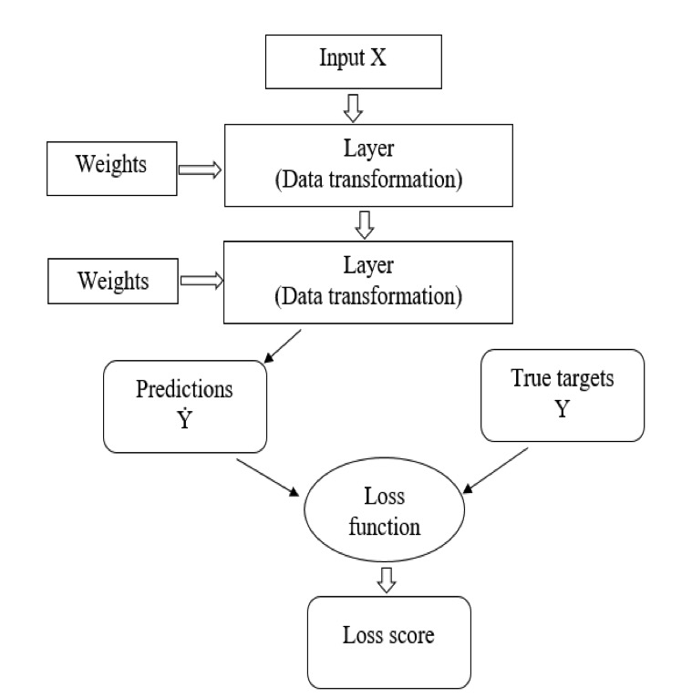
"In general, AI systems work by ingesting large amounts of labeled training data, analyzing the data for correlations and patterns, and using these patterns to make predictions about future states" [Raximov, Kuvandikov and Dilmurod, 2022]. Figure 3 shows that the neural net analyses data and makes predictions. The loss function produces a loss score, which is the result of comparing predicted values to the actual target values. The lower the loss score, the higher the model's accuracy.

1. Mean Square Error
2. Mean Absolute Error
3. Huber Loss
4. Hinge Loss
5. Sigmoid Cross Entropy Loss
6. Weighted Cross Entropy Loss
7. Softmax Cross Entropy Loss
8. Sparse Cross Entropy Loss
9. Kullback-Leibler Divergence Loss

Mean Square Error (MSE)

The Mean Square Error is the most commonly used loss function for regression problems. Mean squared error is defined as the average of the squared differences between the predicted and actual values. Due to the sqaure property of the formula, the resulting value is more penalizing than taking absolute value. The resulting value is always positive. The cost function looks like :

$$\begin{aligned} \text{MSE} = \dfrac{1}{n} \sum_{i=1}^{n} (y_{i} - \hat{y_i})^{2} \end{aligned}$$

where $y_i$ is the true value, $\hat{y_i}$ is the predicted value at the $i^{th}$ rank and $n$ is the number of samples.

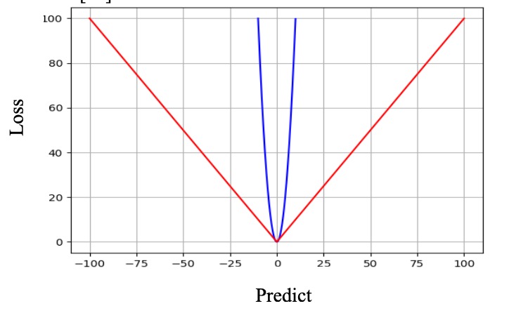
The advantage of using Mean Square Error is penalizes the model for making larger mistakes. Moreover the gradient decent has one global minima and no local minima. The diadvantage of using mean square error is that loss function is not robust for the data that contains outliers.

Mean Absolute Error(MAE)

Mean Absolute Error(MAE) is the another popular cost function in machine learning. It is described as the mean of the absolute discrepancies between the predicted and actual values. It can be shown as :

$$\begin{align} \text{MAE} = \dfrac{1}{n} \sum_{i=1}^{n} | y_{i} - \hat{y_i} | \end{align}$$

where $y_{i}$ is the true value and $\hat{y_i}$ is the predicted value at the $i^{th}$ rank.

The Mean Absolute Error is more robust than Mean Square Error to outlier as shown in the Figure 4. But comparting MAE to MSE, MAE is ... computationally expensive as modulus error is complex to solve compared to square error.(Raximov, Kuvandikov and Dilmurod, 2022). There may be a local minima and the gradient can increase significantly even with minor losses since it remains constant throughout the process, which is not suitable for the learning phase.

Root Mean Square Error(RMSE)

The Root Mean Square is the square root of the mean sqaured Error(MAE). It is defined as :

$$\begin{align} \text{RMSE} = \sqrt{\dfrac{1}{n} \sum_{i=1}^{n} (y_{i} - \hat{y_i})^{2} } \end{align}$$

where $y_{i}$ is the true value, $\hat{y_i}$ is the predicted value at the $i^{th}$ rank and $n$ is the number of samples. The RMSE is the just the square root value of the MSE and it measures the average deviation of the prediction values from the actual values.

Huber Loss

Huber Loss combines the properties of Mean Square Loss and Mean Absolute Loss. Compared to MSE, Huber loss is intended to be more resilient to outliers while possessing smoothness and differentiability. When the error is small, the Huber loss function behaves like the MSE loss function, and when the error is large, the Huber loss function behaves like the MAE loss function. It is less sensitive to large errors. Huber Loss can be written as :

$$\begin{align} f_{n} = \begin{cases} \dfrac{1}{2} (y_{i} - \hat{y}_{i})^{2} &\text{ , if } |{y_{i} - \hat{y}_{i}}| < \varepsilon \\ \\ |{y_{i} - \hat{y}_{i}}| \varepsilon - \dfrac{1}{2} \varepsilon^{2} &\text{ , otherwise} \\ \end{cases} \end{align}$$

The value of $\varepsilon$ is choosen empirically. Choosing different values yield results and the value of $\varepsilon$ can be made based on the best results from the trial and error method. $\varepsilon$ should be small if the data has a lot of outliers and/or a lot of noise.

Regression Loss Function Metrics

The table below shows the environment for thr application of the most popular loss function.

Loss Function	Application
Mean Squared Error(MSE)	General-purpose regression, Model Performance and selection, optimization, Linear Regression Models, neural networks
Root Mean Squared Error (RMSE)	General-purpose regression, model selection, optimization, linear regression, neural networks
Mean Absolute Error (MAE)	General-purpose regression, model selection, optimization, robustness to outliers,time series analysis
Huber Loss	Same as MSE and MAE, with some robustness over noisy data and outliers

Hinge Loss

The hinge loss is a widely used loss function for training classifiers and serves as the de facto maximum-margin classification loss function for Support Vector Machines (SVMs).

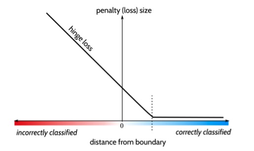
This is the formula for Hinge Loss :

$$\begin{align} \text{hl} = \text{max}(0 ,1 - d \cdot t) \end{align}$$

where $d$ is desired value and $t$ represents the predicted value. The output of the hinge loss is non-negative. If $d \cdot t \geq 1$ indicates that the prediction is correct, the loss is zero. If the value of $d \cdot t < 1$, the prediction is incorrect; the loss is proportional to the distance from the margin (1 in this case). Hinge loss function defines the margin near the decision boundary, and the correctly classified samples in the middle of the two margin boundaries and all misclassified samples have the cost [Wang et al., 2020]. Since hinge loss is non-differentiable, we use a smoothed version to be coupled with optimization functions. The smoothed loss function can be write as

$$\begin{align} \text{shl} = \text{max}(0 ,1 - d \cdot t)^{2} \end{align}$$

The squared hinge loss still penalizes misclassifications, but it does so in a smoother and differentiable manner, making it suitable for use with optimization algorithms that require gradients, such as gradient descent and its variants.

The goal of optimization is to minimize

$$\begin{align} Loss_{Hinge Loss} = \lambda ||w||^{2}+ \left[\dfrac{1}{n} \sum_{i=1}^{N} max\{0, 1 - y_{i}(w^{T} x_{i} - b)\} \right] \end{align}$$

where the parameter $\lambda$ is the size of the margin. The value of $\lambda$ has a tradeoff between the margin size and ensuring that the $x_{i}$ falls on the right side of the margin. If the value of $\lambda$ is too big, it can lead to the items/objects being misclassified based on a vague idea. If its value is too small, it will result in the remotely closed items/objects not classify as objects.

Here are some of the practical applications of hinge loss :

Practical Application	Description
Anomaly Detection	In anomaly detection tasks where the goal is to identify outliers or unusual instances within a dataset. The model is taught to distinguish normal data points from anomalies, aiding in fraud detection, fault diagnosis, or outlier detection in various domains.
Image Segmentation	Hinge loss can be used for single-class image segmentation tasks, where the objective is to separate foreground objects from the background. The model learns to delineate the target object boundaries, facilitating tasks such as medical image analysis, object tracking, or scene understanding in computer vision applications.
Outlier Rejection	In scenarios where the focus is on rejecting outliers or noise while retaining valid data points. By training on the majority class and treating outliers as the minority class, the model learns to differentiate between the normal data distribution and outliers, aiding in robust decision-making and data cleaning processes in various domains, including sensor data analysis, quality control, or anomaly detection in industrial systems.
Customer Behavior Analysis	Hinge loss can be utilized for customer behavior analysis tasks, such as fraud detection or churn prediction in financial services or telecommunications. By training the model normal customer behavior patterns, the model can identify deviations or anomalies indicative of fraudulent activities or potential churn events, enabling proactive risk mitigation strategies and customer retention efforts.
Quality Control	In manufacturing or production environments, hinge loss can be applied for quality control purposes. By training on data representing acceptable product quality, the model can detect deviations or defects in real-time production processes, facilitating early detection of quality issues, reducing scrap rates, and enhancing overall product quality.

Cross Entropy Loss Function

Cross entropy loss, or the logistic loss function, is a cornerstone in binary classification tasks involving two classes, typically labelled as 0 and 1. This loss function proves its prominence by offering a means to gauge the disparity between the actual class and the predicted probability, often expressed as a real number confined within the range of 0 to 1. To harness the efficacy of cross entropy loss, it is customary to employ the sigmoid activation function as the final layer before its application. Through this approach, practitioners effectively quantify the divergence between the predicted probabilities and the true class labels, facilitating the refinement of models to better discern between the distinct classes. The two popular cross-entropy loss functions are

1. Sigmoid Cross Entropy Loss
2. Weighted Cross Entropy Loss

Sigmoid Cross Entropy Loss Function

Sigmoid Cross Entropy Loss is a loss function commonly used in classification tasks, particularly in neural networks where the final layer applies a sigmoid function. The sigmoid cross entropy has independant components that work together to output the loss between the predicted and the actual values. The two components are:

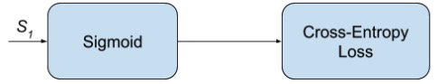
1. Sigmoid Function: The sigmoid function squashes the output of a neural network to a value between 0 and 1, effectively transforming it into a probability.
2. Cross Entropy Loss : Cross entropy loss measures the difference between the predicted probability distribution and the true distribution.

The Sigmoid Function can be written as :

$$\begin{align} f(s_{i}) = \dfrac{1}{1 + e^{- s_{i}}} \end{align}$$

Cross Entropy Loss Function can be written as. :

$$\begin{align} CE = - \sum_{i=1}^{C' = 2} t_{i} log(f(s_{i})) - (1 - t_{1}) log(1 - f(s_{1})) \end{align}$$

In this formula the terms mean the following:

• $C'= 2$ represents the number of classes in the classification problem.
• $t_{i}$ represents the ground truth label for class $i$.
• $f(s_{i})$ represents the predicted probability for the class $i$ using the sigmoid function.
• Finally the sum is taken over all the classes.

The binary cross entropy and the sigmoid function complement each other in the output layer for the following reasons :

1. Probability-based Output: The sigmoid function converts the results into probability, which is bounded between 0 and 1. The binary cross-entropy function fits this feature and is intended to evaluate the difference between expected probability and actual binary labels.
2. Effective Learning Gradient: For learning to be effective, the loss function's gradient should be practical and easily computable. The binary cross-entropy and sigmoid functions' mathematical characteristics lead to a positive gradient product, making training optimization easier.
3. Penalize for Incorrect Predictions: The sigmoid and cross-entropy functions penalize incorrect predictions confidently. Because the sigmoid function is logarithmic, the model makes an incorrect prediction with high certainty. This improves the model's generalization performance by encouraging it to be more circumspect and less self-assured when generating predictions.

The practical application of the Sigmoid Cross Entropy Function are :

Application	Description
Binary Classification	Used for tasks like spam detection or medical diagnosis, where the model predicts the probability of belonging to one of two classes.
Multi-label Classification	Applied in scenarios where each sample can belong to multiple classes simultaneously, such as tagging images with multiple labels.
Anomaly Detection	Utilized to detect rare instances or outliers in a dataset, helping identify abnormal behaviour or events in cybersecurity or industrial systems.
Imbalanced Classification	Addresses class imbalance issues in datasets where one class is significantly more prevalent, improving performance on minority classes.
Recommender Systems	Employed to predict user preferences or ratings for items in recommender systems, enhancing personalized user recommendations based on their preferences.

Weighted Cross Entropy Function

Weighted cross-entropy loss is a variant of the standard cross-entropy loss function that introduces class weights to address the class imbalance in binary classification problems. This is useful in situations where the distribution of the samples is imbalanced. In order to solve this problem, weighted cross entropy loss computes the loss function using distinct weights for the positive and negative classes. The relative significance of accurately identifying each class is reflected in these weights. The positive class, or minority class, is usually given more weight than the negative class or dominant class. The Weighted Cross Entropy Loss function is mathematically expressed as :

$$\begin{align} L = -(w_{i} \cdot y log(p) + w_{i}(1-y) log(1-p)) \end{align}$$

where

• $p$ is the predicted probability of the positive class.
• $w_i$ is the weight assigned to the $i^{th}$ sample
• $y$ is the true label

The Weighted Cross Entropy Function is a good loss function because:

1. Addresses Class Imbalances: Weighted Cross Entropy Loss tackles imbalanced datasets by assigning different weights to classes, emphasizing the minority class.
2. Customizable Weights: The weights can be adjusted based on dataset characteristics and class importance, offering flexibility and adaptability. Weighted Cross Entropy Loss improves model robustness and performance on unseen data by mitigating bias towards the majority class.

The practical application of the Weighted Cross Entropy Function are :

Application	Description
Imbalanced Classification	Weighted Cross Entropy Loss is particularly useful for addressing class imbalance in datasets by assigning higher weights to minority classes, improving model performance.
Object Detection	Used in object detection tasks where the presence or absence of objects in images needs to be accurately classified, with adjusted class weights to handle imbalanced classes.
Medical Diagnosis	Applied in medical diagnosis to predict the presence or absence of diseases, with adjusted class weights to prioritize correct classification of rare or critical conditions.
Fraud Detection	Utilized in fraud detection systems to identify fraudulent transactions or activities, with adjusted class weights to focus on correctly detecting fraudulent instances.
Customer Churn Prediction	Employed in customer churn prediction models to forecast the likelihood of customers leaving a service or subscription, with adjusted class weights to improve prediction accuracy.

Softmax Cross Entropy Loss

The softmax cross-entropy loss is a commonly used loss function for multiclass classification problems. The primary distinction between this loss function and the sigmoid cross-entropy function lies in substituting the sigmoid function with the softmax function, which is tailored explicitly for resolving multiclassification challenges. When computing the softmax loss function, the values in a vector are normalized into a probability distribution consisting of values between and 1, with the sum of probabilities equal to 1. The softmax function is defined as :

$$\begin{align} p_{i} = \dfrac{e^{z_{i}}}{\sum_{j=1}^{N} e^{z_{j}}} \end{align}$$

where

• $p_i$​ is the probability of class $i$,
• $z_i$​ is the raw score for class $i$
• $N$ is the total number of classes.

The Softmax cross-entropy loss function, derived as probabilities by the softmax function, assesses the disparity between predicted and actual probability distributions.. The softmax function is presented mathematically as :

$$\begin{align} L = - \sum_{i=1}^{N} y_{i} \cdot log \left(\dfrac{e^{z_{i}}}{\sum_{j=1}^{N} e^{z_{j}}} \right) \end{align}$$

where

• $y_i$​ is the true probability distribution (often represented as a one-hot encoded vector) for class $i$
• $z_i$​ is the raw score for class $i$.

Given that numerous practical challenges, such as semantic segmentation and text mining, involve multi-classification tasks, the softmax cross-entropy loss has emerged as a predominant loss function in deep learning. This trend is evident across a plethora of deep-learning literature.

Here's the information presented in a simple table format:

Application	Description
Multiclass Classification	Softmax Cross Entropy Loss is commonly used in multiclass classification tasks where samples belong to one of multiple classes, enabling the model to output class probabilities that sum up to 1.
Handwritten Digit Recognition	Applied in tasks such as recognizing handwritten digits, where each input image corresponds to a single class label out of a predefined set (e.g., digits 0-9), facilitating accurate classification.
Language Identification	Utilized in language identification systems to determine the language of a given text sample from a set of possible languages, with Softmax Cross Entropy Loss ensuring probabilistic predictions for each language.
Facial Expression Recognition	Employed in facial expression recognition applications to classify facial expressions (e.g., happy, sad, angry) from images or videos, with Softmax Cross Entropy Loss facilitating multiclass classification of expressions.
Sentiment Analysis	Used in sentiment analysis tasks to classify text documents (e.g., customer reviews, social media posts) into multiple sentiment categories (e.g., positive, negative, neutral), enabling accurate sentiment classification.

Impact of Loss Functions on Model Behavior:

Choosing the appropriate loss function in machine learning is paramount as it directly impacts the model's performance, generalization, and robustness. The loss function is a critical component in the optimization process, guiding the model to minimize thediscrepancy between predicted and actual values during training. It is important to understand the use case the type of the problem the user is trying to solve. Different tasks and datasets require different loss functions, each tailored to the specific characteristics of the problem at hand. For instance, classification tasks may benefit from cross-entropy loss, while regression tasks might require mean squared error. Selecting an inappropriate loss function can lead to suboptimal model performance, slower convergence, or even divergence during training. Moreover, certain loss functions are more sensitive to outliers, class imbalances, or noisy data, highlighting the need for careful consideration when choosing the appropriate loss function. Ultimately, the choice of loss function profoundly influences the effectiveness and reliability of machine learning models, underscoring its importance in developing successful and robust AI systems. It is also important to do due diligence and analysis over interaction between different components of the machine learning algorithm for a effectively and robust output.

Conclusion

Choosing the correct loss function in machine learning is crucial as it directly influences how a model learns and performs on a given task. The loss function guides the optimization process, helping the model adjust its parameters to minimize errors during training. Different tasks and datasets may require different loss functions tailored to their specific characteristics. In regression problems, metrics like Mean Squared Error (MSE), Mean Absolute Error (MAE), and Root Mean Squared Error (RMSE) are commonly used to evaluate the performance of predictive models. MSE measures the average squared difference between the predicted and actual values, penalizing more significant errors more heavily. Conversely, MAE computes the average absolute difference between predicted and actual values, providing a more interpretable measure of error. RMSE is the square root of MSE, which measures the typical magnitude of the error. Ultimately, the choice of metric depends on the specific characteristics of the dataset and the priorities of the regression task at hand. In case of Hinge loss, for instance, is commonly employed in binary classification tasks, particularly with Support Vector Machines (SVMs). It penalizes misclassifications and encourages correct classification by maximizing the margin between classes. The Sigmoid Cross Entropy Loss Function is often utilized in binary classification problems where the model output needs to be interpreted as a probability. It computes the cross-entropy loss between the predicted probabilities and the true binary labels, with the sigmoid activation function ensuring that the predicted probabilities are between 0 and 1. Weighted Cross Entropy Loss Function extends cross-entropy loss by assigning different weights to different classes. This is useful when dealing with imbalanced datasets, where certain classes may be more important or prevalent than others. Lastly, Softmax Cross Entropy Loss is commonly used in multi-class classification tasks. It computes the cross-entropy loss between the predicted class probabilities (obtained through the softmax activation function) and the true one-hot encoded class labels. Each of these loss functions serves a specific purpose in evaluating the performance of classification models, depending on the task's nature and the dataset's characteristics.

Biblography

• [Kavzoglu, 2009] Kavzoglu, T. (2009). Increasing the accuracy of neural network classification using refined training data. Environmental Modelling & Software, 24(7), pp.850–858. doi:https://doi.org/10.1016/j.envsoft.2008.11.012
• [Dongare, Kharde and D.Kachare, 2008] Dongare, A.D., Kharde, R.R. and D.Kachare, A. (2008). Introduction to Artificial Neural Network. Certified International Journal of Engineering and Innovative Technology (IJEIT), [online] 9001(1), pp.2277–3754. Available at: https://citeseerx.ist.psu.edu/document?repid=rep1&type=pdf&doi=04d0b6952a4f0c7203577afc9476c2fcab2cba06.
• [Hashemi-Pour, Zola and Vaughan, n.d.] Hashemi-Pour, C., Zola, A. and Vaughan, J. (n.d.). What is a backpropagation algorithm and how does it work? [online] TechTarget. Available at: https://www.techtarget.com/searchenterpriseai/definition/backpropagation-algorithm.
• [Jensen, 2023] Jensen, K. (2023). An Introduction to Reinforcement Learning for Neuroscience. [online] Available at: https://arxiv.org/pdf/2311.07315.pdf [Accessed 31 Mar. 2024].
• [Krogh, 2008] Krogh, A. (2008). What are artificial neural networks? Nature Biotechnology, [online] 26(2), pp.195–197. doi:https://doi.org/10.1038/nbt1386.
• [Terven et al., 2023] Terven, J., Cordova-Esparza, D., Ramirez-Pedraza, A. and Chavez-Urbiola, E. (2023). LOSS FUNCTIONS AND METRICS IN DEEP LEARNING. A REVIEW UNDER REVIEW IN COMPUTER SCIENCE REVIEW. [online] Available at: https://arxiv.org/pdf/2307.02694.pdf.
• [Raximov, Kuvandikov and Dilmurod, 2022] Raximov, N., Kuvandikov, J. and Dilmurod, K. (2022). The Importance of Loss Function in Artificial Intelligence. In: IEEE. [online] 2022 International Conference on Information Science and Communications Technologies. IEEE, pp.1–3. doi:https://doi.org/10.1109/ICISCT55600.2022.10146883.
• [Wang et al., 2020] Wang, Q., Ma, Y., Zhao, K. and Tian, Y. (2020). A Comprehensive Survey of Loss Functions in Machine Learning. Annals of Data Science. doi:https://doi.org/10.1007/s40745-020-00253-5.
• [Ciampiconi et al., n.d.] Ciampiconi, L., Elwood, A., Leonardi, M., Mohamed, A. and Rozza, A. (n.d.). A survey and taxonomy of loss functions in machine learning. [online] Available at: https://arxiv.org/pdf/2301.05579.pdf.